
Yap Chuan Fu
Research Associate at The University of Manchester. I enjoy solving problems using computers and mathematics.
Linear Regression Crash Course
Theory dive with application in Python - 35 min read
Published Dec 11, 2022
tldr; This will be a crash course on Linear Regression for statistical analysis with code implementation in Python. It will have minimal explanation on the maths. Feel free to navigate to make use of the Table of Contents on the left sidebar to skip to section of interest which would have theory and code on them, or click here for code compilation.
Prologue
Linear regression is what I would describe as the ‘swiss army knife’ of statistical models or the ‘Canon in D’ of modelling if you will. This simple equation: \begin{equation} y = mx+c \end{equation} is often undersold when you were first taught it in high school level (or earlier I don’t know what kind of education you had). We were told y is what we want to map to using a line of best fit with point x, with which we use to compute slope/gradient/rate of change m along with the intercept c. As we move up in education levels, its significance is elevated and the equation is rewrote as the following: \begin{equation} Y_i = \beta_0 + \beta_1 X_i + \epsilon_i \end{equation} This time, it is introduced as a statistical tool with the usual package of p-value in it along with an error term. This form of equation is also known as simple linear regression (SLR), for it has single independent variable X relating to single dependent variable Y.
While this equation have been around for hundreds of years, its application is becoming more widespread across scientific research as well as analytical departments of businesses in recent century. The reason for this is the (extreme) generalisation this equation allows for (along with its interpretability), which is normally not taught to us, at least not in an adequate manner.
By generalisation, I mean how data can be generalised in this linear manner when not all data relationship is linear, as well as the ease of modification to the model to expand on its usage.
We are typically just told the dry version of linear regression usage which is more or less:
A deterministic model describing the linear relationship between two variables X and Y.
Usually, X is known as the independent variable and Y is the dependent variable, because its value depends on another variable(s) (e.g. X) or parameter(s). There are alternative semantics used by different fields such as in machine learning, X is feature and Y is target, more can be read on this wiki page.
dependent variable = response = outcome
independent variable = predictor = features
This blogpost will cover the basic of linear regression and some of its extensions that makes it the swiss army knife of statistical models. Another name for this modelling approach which I prefer is linear model because regression is an approach in machine learning which predicts continuous outcome, linear models can be generalised beyond that as some of you would be familiar with logistic regression which predicts binary outcomes.
This post is the cumulation of knowledge I have gathered from STAT501, a PennState course module, Statistical Rethinking, a wonderful statistics textbook and Coursera’s Machine Learning course (pre 2022 update) by Andrew Ng. This blogpost also serves as my notepad for collating the notes I have taken from these sources as well as implementation in Python.
What is Simple Linear Regression (SLR)?
\begin{equation} Y = \beta_0 + \beta_1 X + \epsilon \end{equation}
- Y, is the response/dependent variable
- X, is the predictor/independent variable
- \(\beta_0\), is the intercept
- \(\beta_1\), is the regression coefficient/slope/gradient
- ϵ, is the normally distributed random error
This is a ‘simple’ linear model because it has one predictor variable and one response variable. For multiple linear regression (MLR) with > 1 predictor variable, go here.
Assumptions/Conditions for SLR to work
- Linear relationship/function
- Independent errors
- Normally distributed errors
- Equal variances
It is an acronym (LINE) to help you remember, since the model gives you line of best fit.
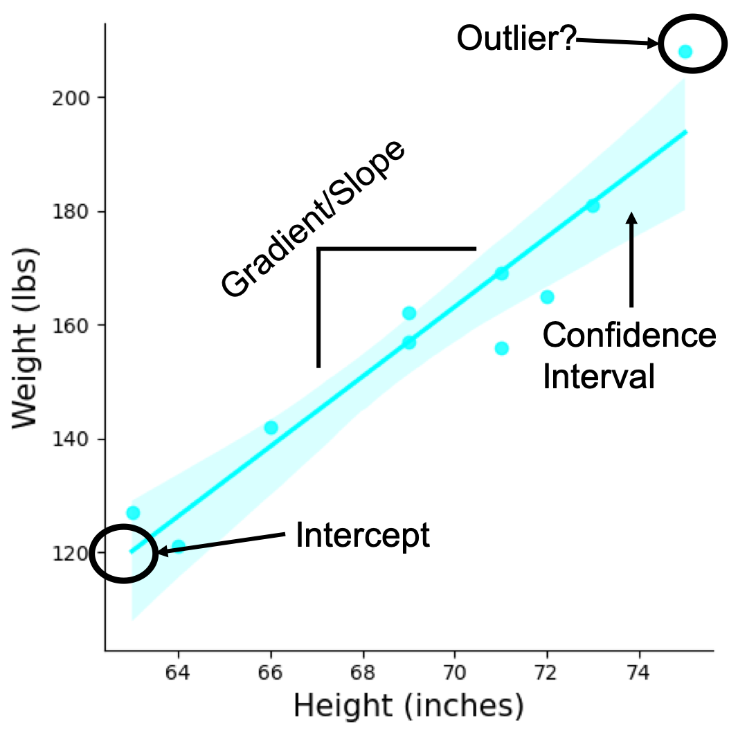
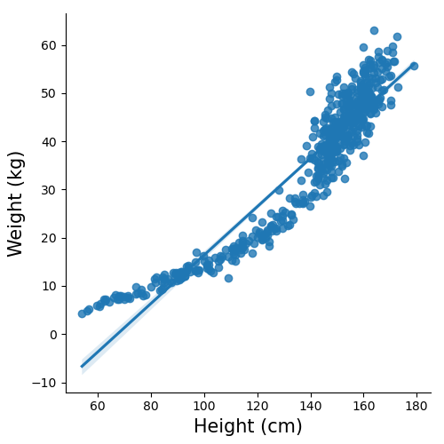
Plot above is a brief anatomy of a SLR model highlighting the components from the equation. Note, I have plotted the data points as well as the line of best fit resulting from the model. Whenever possible visualisation of the model along with the data points is important when the analysis is being presented. For example in the plot above we can see there is a potential outlier. In another example plot below, while you can get a straight line to fit, it might not be best representation of the data which shows a curvature.
Above plots can be made easily using seaborn with the following code sns.lmplot(x, y, data)
Interpretation of SLR
Slope/Gradient/Regression Coefficient
β1=1, 1 unit increase in X results in 1 unit increase in Y
- We expect the mean response Y to increase/decrease by estimated \(\beta_1\) unit for every one unit increase in X. Substitute X with 1 in the equation and it’ll make sense in the equation.
- In some cases we standardise the data X by subtracting the data vector X by its mean and dividing by its standard deviation; in code
(X-X.mean())/X.std()assuming X is an array. The coefficient interpretation changes to mean change in standard deviation in the association between X and Y.
Intercept
mean value of Y
- The mean value of Y when X is zero. Substituting X with 0 and it would make sense in the equation. Usually data you are analysing the value of X theoretically cannot be zero, for example in height and weight relationship, neither variables can be zero. So to get an accurate interpretation for situations like this, we can mean-centre the X prior to model fitting, and the intercept would give the mean Y of the data when X is at its mean. Mean-centre means subtracting data vector X with the mean of X; in code
X - X.mean(), assuming X is an array.
Why use SLR??
The simple interpretation of unit increase from coefficient explained above is one the reasons on why we use SLR, but the other reasons are:
Hypothesis testing
null hypothesis, β1=0
alternative hypothesis, β1=/=0
Hypothesis testing in frequentist statistics require a null hypothesis, which is something we want to disprove. With SLR, the null hypothesis is β1=0, therefore the thing we want to show is that β1=/=0, which is the alternative hypothesis. This would demonstrate that there is an association between X and Y. This also means that a change in X results in a meaningful (or statistically significant) change in Y.
We can do this using statsmodels, for example if we want investigate relationship between heigh and weight.
Here’s what the first 5 rows of the 2 column data looks like:
| ht | wt |
|---|---|
| 63 | 127 |
| 64 | 121 |
| 66 | 142 |
| 69 | 157 |
| 69 | 162 |
Where ht is height, and wt is weight.
import pandas as pd
import statsmodels.api as sm
# load data
df = pd.read_csv("data/student_height_weight.txt", sep='\t')
## setting the variable names
## For X we need to run this function to generate a columns of 1 to represent the intercept
## you can check using X.head()
X = sm.add_constant(df.ht)
y = df.wt

## build OLS object, which stands for ordinary least square
## a type of regression model fitting method.
model = sm.OLS(y, X)
## fit the model
results = model.fit()
Alternatively, we can make use of formula method of building linear models, which feels more convenient as we don’t need to use the add_constant function to generate intercept as it would do it for us.
## this is so simple where we don't need to include intercept and error term
## and we would need to use the actual variable/column name within the data
## this is of course assuming data have been loaded with pandas
model = smf.ols(formula='wt ~ ht', data=df)
## so the equation is basically Y ~ X and we have chose wt as Y and ht as X in this model.
results = model.fit()
To view the outcome of fit execute print(results.summary()) and we get the following table with lots of information.
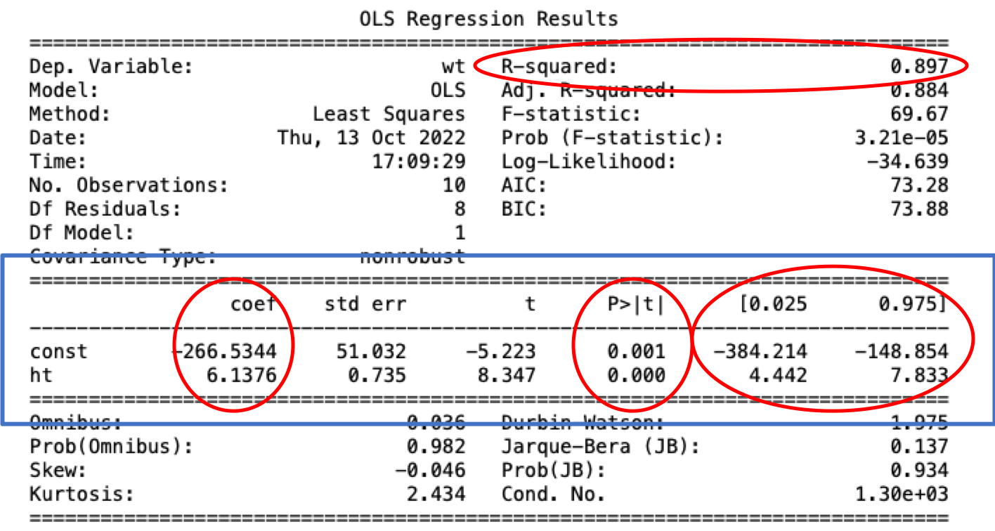
I have circled the immediate things that would be of interest for simple models, everything else is more advanced for further model diagnosis if necessary.
From top to bottom and left to right, things of interest are:
- \(R^2\) (R-squared), Coefficient of Determination
- explains variation in Y explained by the model, values ranges from 0-1, and higher value is better. But a good value depends between research field.
- Coefficient (coef)
- this was as explained above, where const correspnods with the intercept’s coefficient, and ht is X of this model.
- P-value (P >|t|), the all fabled measure of statistical significance
- the essential ingredient of frequentist statistics where values <0.05 implies statistical significance where null hypothesis is disproven and (usually) therefore an important finding.
- 95% Confidence Interval (0.025, 0.975)
- The measure of confidence on the estimated coef. That is 95% of such confidence intervals in repeated experiments will contain the true value.
- The alternate more popular interpretation is the a more Bayesian interpretation,which is we are 95% sure the estimated coef is between these values.
Normally, when we report our results, on top of plotting, we would highlight the three things within the blue box, which are coefficient value, p-value and the confidence interval.
CAUTION:
- large \(R^2\) does not necessarily mean it is a good model.
- low/significant p-value is not useful if the coefficient is low.
Prediction
Arrival of big data allowed for the boom of machine learning, and linear model is one of the algorithms used in supervised learning for prediction purposes. Models trained with statsmodels can be used for prediction as well using predict function on the fitted model object, e.g. results.predict(new_X).
The more popular and convenient option for prediction is with scikit-learn. Example code:
import pandas as pd
from sklearn.linear_model import LinearRegression

## load data
hw = pd.read_csv("data/Howell1.csv", sep=';')

## note this is a different dataset from earlier hence the different variable names
## set variables names
X = hw[['height']]
y = hw[['weight']]
## fit and train model
lm = LinearRegression()
lm.fit(X,y)
The above code would give you a trained linear model for prediction when you have new data, e.g. lm.predict(new_X), you would then be able to score it using any metric you need, and scikit-learn provides many of it on their website.
If you were wondering about the intercept of the model, by default sklearn includes the intercept, but you can exclude it by running LinearRegression(fit_intercept=False) when creating the object.
Disclaimer, there is more to good machine learning practice than just fitting a model and scoring it.
How to know SLR is working?
We have learned what is SLR and what it’s used for, now we learn how we know it is working as intended.
Coefficient of Determination, \(R^2\)
This gives the measure of how much variance the response variable is explained by the model. Higher value would usually imply a good model, however this should always be accompanied with a visual inspection with a scatter and linear plot as a single data-point can impact the \(R^2\).
Making sure assumptions are not violated
The LINE assumption is of extreme importance when it comes to hypothesis testing. The statistical significance would not hold if any of the assumption is violated, because these tests were developed with these assumptions in mind. When it comes to prediction, overfitting and underfitting is priority over model assumptions.
NOTE: it is not the end of the world if some of these are violated as they can be fixed with data transformations (results not guaranteed).
There are various tests for this, coming in quantitative and qualitative flavors. I personally prefer the visualisation approach for this, with these three that covers all the assumptions:
1) Residuals vs Fits plot
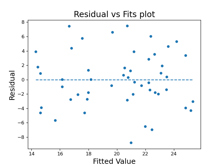
This is a plot where the x-axis is the fitted values, values predicted by the model on data and y-axis is the residual of the model, where residual is the difference between actual Y and predicted Y. This lets us check for linear and equal variance assumption.
To plot this:
## load data and fit model
alcohol = pd.read_csv("data/alcoholarm.txt", sep="\s+")
X = sm.add_constant(alcohol.alcohol)
y = alcohol.strength

model = sm.OLS(y, X).fit()

## extract values to plot
fitted = model.predict(X) #get predicted/fitted values
resid = model.resid ## gets us the residual values

## scatter plot
sns.scatterplot(fitted, resid)
# np is numpy package used to find min max value
plt.hlines(y=0, xmin = np.min(fitted), xmax=np.max(fitted), linestyle="--")
When the residual bounces randomly around the horizontal (residual=0) line such as plot above, it would mean the linear assumption is reasonable. If it was violated, it would have an obvious pattern such as a fixed line or wave for example.
When the residual forms a approximate ‘horizontal band’ along the horizontal line, it would mean the equal variance assumption holds. If it was violated, it would form a cone in either direction.
2) Residual vs Order plot
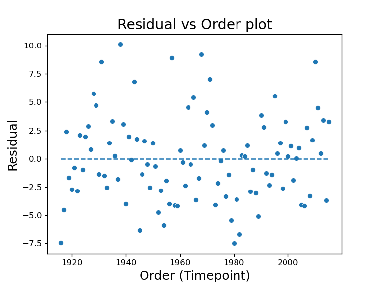
This is a plot where the x-axis is the order of the variable was collected, and y-axis is the residual of the model, where residual is the difference between actual Y and predicted Y. This lets us check for independence assumption. This is mostly use when you have a time series data where the order of the data is known, and we want to know if the response variable is dependent on the time variable. This plot is really only appropriate when we know order the data is collected such as the time.
To plot this:
## load data and fit model
eq = pd.read_csv("data/earthquakes.txt", sep="\t", index_col=0)

X = sm.add_constant(eq.index)
y = eq.Quakes

model = sm.OLS(y, X).fit()

## extract values to plot
resid = model.resid

## scatter plot
sns.scatterplot(eq.index, resid)
# np is numpy package used to find min max value
plt.hlines(y=0, xmin = np.min(eq.index), xmax=np.max(eq.index), linestyle="--")
When there is a random pattern such as the residual vs fit plot, it would mean no serial correlation or dependence. The example plot shown reveals a wave pattern in the data points, which means there is a trend of the response variable dependent on time.
When this happens, SLR is no longer the ideal analysis tool for this dataset, we should instead move on to time series analysis using for example autoregressive models.
3) Normal probability plot of residuals (QQ-plot)
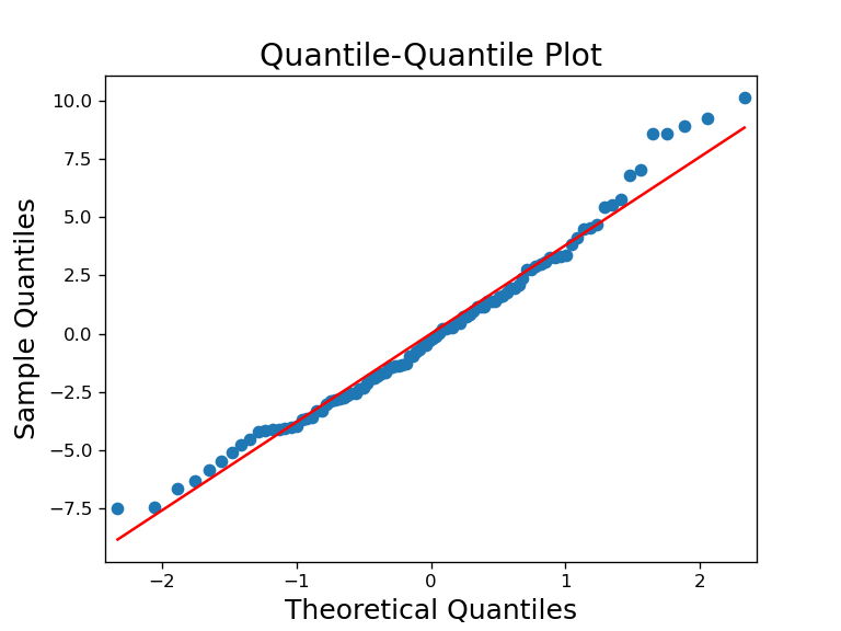
This plot shows the residual’s quantile against a theoretical ‘normal’ quantiles. This lets us check the normality assumption. If the data or residuals are normal, it would match up closely with the theoretical line. Deviations of data points from the red line would indicate non-normal residuals/data.
This can be plotted as such:
fig = sm.qqplot(resid, line="s") ## built into statsmodel
Above are some of the easy checks for linear model assumptions. statsmodels have more built in functions for other plots and quantitative tests, for example this page covers other plots that can be used to diagnose/investigate the model, as well as a simple one line code that plots several things, sm.graphics.plot_regress_exog(fitted_model, "variable_of_interest")
How to estimate the parameters in SLR?
This section is probably not of interest to many since I have already shown how statsmodels and scikit-learn can fit the model with one line. But if you are interested in how this is done, below are two methods that are used for linear model fitting.
REMINDER: regression coefficient = slope = gradient, is the parameters in SLR model.
In SLR, when estimating parameters the most common method is to find parameters that would produce the minimum sum of squared residuals. This method is known as ordinary least squares (OLS).
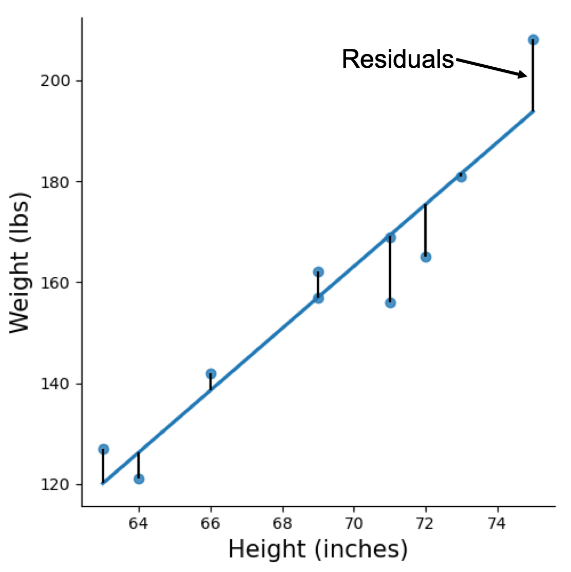
Figure above visualises the residuals in a SLR model, which is the gap between predicted value (line) and actual value (dot).
Linear Least Square/Normal Equation
With OLS, there is a closed form solution for this:
\begin{equation} \hat{\beta} = (X^TX)^{-1}X^Ty \end{equation}
Where
- \(\beta\), the model coefficients being estimated
- \(X\), the independent variable matrix
- \(X^T\), transposed independent variable matrix
- \(y\), the dependent variable
- the superscript of -1, is notation of inverse matrix
To solve this, you to apply some linear algebra. In Python you can do it with numpy.
Gradient Descent
This method can be quite involved and deserves a post of its own, so I would just mention that gradient descent is or a variation of it, the stochastic gradient descent are the commonly used algorithms to estimate parameters in SLR.
Multiple Linear Regression
Now we move beyond the ‘simple’ in SLR and include more than one independent variable in the model, with that we get Multiple Linear Regression (MLR).
More information is ‘always’ helpful when it comes to modelling, which is why MLR is preferred if there is extra variables available.
alwayshave been placed in quotes because there can be cases that more information just leads to an overfit and misinformed model. Model building should always be done with some level of caution instead of putting all the data in and expect the best. An age old wisdom in model building is ‘garbage in, garbage out’.
To build the MLR model with statsmodels:
## assuming data is loaded with pandas as `df`
## given generic X and Y, where X_1, X_2, X_3 are different variables
X = sm.add_constant(df[["X_1", "X_2", "X_3"]])
y = df.Y

# build OLS object
model = sm.OLS(y, X)
## fit the model
results = model.fit()
With statsmodels’s formula option:
model = smf.ols(formula='Y ~ X_1 + X_2 + X_3', data=df)
results = model.fit()
And with sklearn:
## assuming data is loaded with pandas as `df`
## set variables names
X = df[["X_1", "X_2", "X_3"]]
 # the different data indexing is to play nice with sklearn dimensionality requirement
y = df[['Y']]
## fit and train model same as before
lm = LinearRegression()
lm.fit(X,y)
Below are two statistical explanations on why using MLR is useful.
Control/Adjust/Account for Confounders
The most commonly used if not most useful reason to have additional predictor variables in linear models is to allow the model to control/adjust/account for confounders. I use the three phrases: control, adjust and account because depending on what field of research you are in, different semantics are used.
What is a confounder and why should we control for it?
A confounder is a variable that has an effect on both dependent and independent variable. This allows the confounders to hide important effects and potentially produce false ones.
By including the confounder in the model, we have controlled for it. This would “separate” their effects from the other independent variables.
Furthermore, it could also be that other variable(s) are known to associated with dependent variable (but not to independent variable), we could also include it in the model, this is referred as ‘conditional analysis’, where we condition the model on the known variable to analyse other variables. This would have the same effect as before, where we can then see effect of the new variable being studied after the known variable’s effect is accounted for.
Given the extra variables in the model, the interpretation is updated slightly as such:
each \(\beta\) unit results in a unit change in mean response Y provided all other predictors are held constant.
To work with an example that would be easy to understand, let’s continue with the theme of height. The fantasy race dwarves are known to be shorter than humans, and visually pudgy, so I am assuming for them to have higher BMI than humans. If we were in Middle-earth collecting census, without accounting for race, our weight/height data would be rather strange.
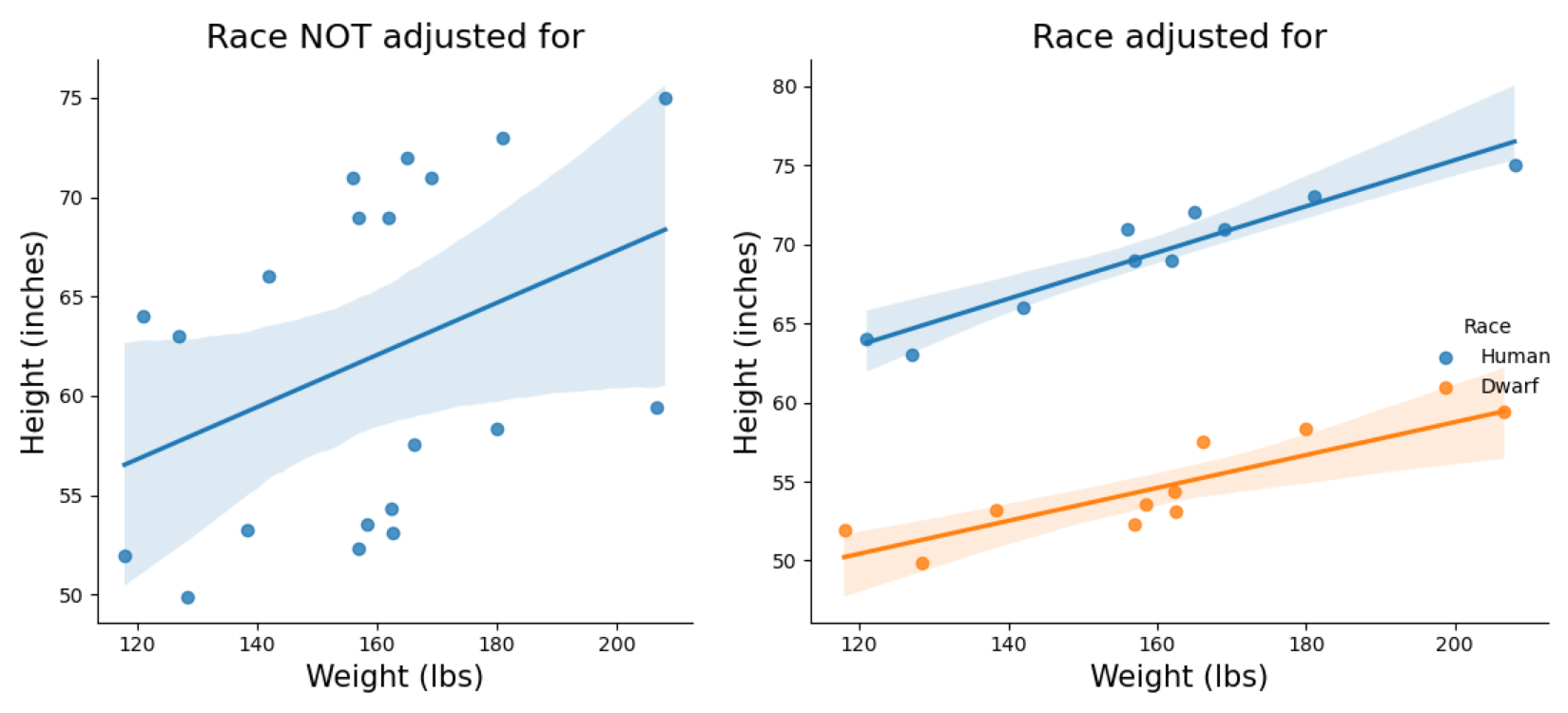
To plot figure on the right:
sns.lmplot(x='weight',y='height', hue='Race', data=DATASET)
## hue option highlight variable of interest to plot separately within the same figure
Plot on the left shows what happens to our model when we fail to account for race, and used only one variable. The plot on the right shows two clear parallel line between them when accounting for race.
i.e. the model on the right is:
\begin{equation} weight = \beta_0 + \beta_1 height+ \beta_2 race \end{equation}
This toy model can be “thought of” as having ‘two’ models in one. That is one regression model for each race. Race here is a categorical variable which would be represented with 0 or 1 for either races, e.g. 0 for dwarf, 1 for human. When we want to compute height of human, \(\beta_2\)’s value would be added to the calculation of weight, and when computing for dwarf’s weight, \(\beta_2\)’s value is not included.
E.g.
For human (coded as 1):
\begin{equation} weight=\beta_0 + \beta_1 height+ \beta_2 1 \end{equation}
For dwarf (coded as 0):
\begin{equation} weight=\beta_0 + \beta_1 height+ \beta_2 0 \end{equation}
0 multiply \(\beta_2\) is still 0. so the outcome of weight is just \(\beta_0\) + \(\beta_1\)*height
So this model would compute the overall relationship between height and weight (in \(\beta_1\)), and include the effect of race within it (in \(\beta_2\)). If the labels of race is flipped, 1 for dwarf and 0 for human, \(\beta_2\) would just have a negative value, but results is still the same.
The previous interpretation of coefficients have also changed with regards to categorical variables, but only slightly. Instead of per unit increase, it is simply the mean difference between the two ‘categories’ or ‘groups’ with regards to the response variable. The hypothesis test is now if the two groups are ‘significantly’ different after accounting for the other variable.
Above is an easy to understand/visualise example with categorical predictors (dwarf vs human) where we can see an additive effect of the extra ‘race’ variable.
When using categorical predictors in a linear model, stats packages would assign one of the values as a reference/template/contrast (once again it is field specific for the semantics). It would code the reference value 0 and 1 for the other during modelling. For example, in the example above, dwarf is the reference variable, and the human variable would have an unit increase in height given the same weight value between the two races.
To make it clear, use of extra variables in linear models is not limited to categorical predictors as per example above, quantitative variables (continuous or discrete) can be used in the same manner. Further, you can include >2 variables in the model despite the example, e.g. for height weight relationship, you can include age, and sex.
On the note of categorical predictors, they have to be converted to numerical values prior to model building manually, with the exception of statsmodels formula.
To convert it:
from sklearn import preprocessing
le = preprocessing.LabelEncoder()
plothw["coded_Race"] = le.fit_transform(plothw["Race"]) # this creates new column in the dataframe

# OR if you know the variable's values
plothw["coded_Race"] = plothw["Race"].map({"Human":1, "Dwarf":0})
Conveniently with formula. simply by appending C():
model = smf.ols(formula = "height ~ weight + C(Race)", data=plothw)
results = model.fit()
CAUTION: the number of predictors (p) we can have in a model is limited by the number of samples (n). That is, we cannot have a
p>nsituation in our models. For statistical reason because we would not have enough degrees of freedom to estimate the parameters in the model. In machine learning, for linear models, this would likely lead to overfit and it learns the noise and reduce model generalization in prediction.
Regressing Out Variable
Above examples uses multiple variables within one model to account for the variables, but we could also divide up the variables into more than one model, e.g. the height ~ weight + race model could be divided into a two step model.
For this, we can first fit height ~ race, and extract the residuals, and fit residuals ~ weight. The final model would have equivalent coefficient for height as the full model’s height coefficient. This process of fitting variable(s) and extracting the residuals is known as “regressing out” variable. The idea is that, everything accounted for by the first set of variables are already in the model, and the residuals are not accounted for (not explained by the variables), so we can pass that on to be modeled by a separate model.
This process of regressing out variable(s) serves no obvious purpose when we can build one big model using linear model, but comes in handy when dealing with multiple model within your statistical analysis pipeline. For example, we know some variables have clear linear relationship but other models have no easy way to account for them, we can regress out the variable with linear relationship and extract the residuals to be passed onto the other modelling frameworks as target variables.
In machine learning, this is equivalent to stacking ensemble framework, where we can use linear model to extract the linear relationship and pass on the residuals to other algorithms capable of handling non-linear relationship such as random forest.
Interaction Models
When the importance/effect of one variable depend upon another variable, this is known as interaction effect. Models that include this would then be interaction models, and as before, the model can include >1 interaction effect within it.
To build an interaction model, we multiply the two variables being investigated and use the resulting values as a new variable in the model. This newly created variable is also known as an interaction term. In machine learning field, this variable creation step is known as feature engineering.
Unfortunately no clever examples from Middle-earth.
E.g. we want to investigate the interaction of variable \(X_1\) on \(X_2\) on Y.
\begin{equation} Y=\beta_0 + \beta_1 X_1+ \beta_2 X_2 + \beta_{1,2}(X_1X_2) \end{equation}
Where \(X_1X_2\) is the aforementioned newly created interaction term via multiplication.
To do this in statsmodels:
## assuming data in df
# first make the interaction term
df["interaction_term"] = df["X_1"] * df["X_2"]

# the rest is same as MLR building
X = sm.add_constant(df[["X_1", "X_2", "interaction_term"]])
y = df.Y

# build OLS object
model = sm.OLS(y, X)
## fit the model
results = model.fit()
With formula option:
model = smf.ols(formula='Y ~ X_1 * X_2', data=df)
results = model.fit()
This above option, would automatically create a new variable for you in the model, and it would come out as \(X_1:X_2\), where “:” means interaction between the two variables. If for some reason, you don’t want the \(X_1\) and \(X_2\) in the model, you can just write Y ~ X_1:X_2.
Again with sklearn:
## same as above
df["interaction_term"] = df["X_1"] * df["X_2"]

# the rest is same as MLR building
X = df[["X_1", "X_2", "interaction_term"]]
 # the different data indexing is to play nice with sklearn dimensionality requirement
y = df[['Y']]

## fit and train model same as before
lm = LinearRegression()
lm.fit(X,y)
With formula option:
model = smf.ols(formula='Y ~ X_1 * X_2', data=df)
results = model.fit()
How do we make sense of the interaction term? Before we get into the equation, let’s visualise some made up examples, as I have said several times, visualisation is always the easiest way to make sense of small linear models. With interaction term, the same applies, and to make it easier for visualization categorical predictors will be used for \(X_2\), and to make it even easier, it will be fruits, apple and orange.
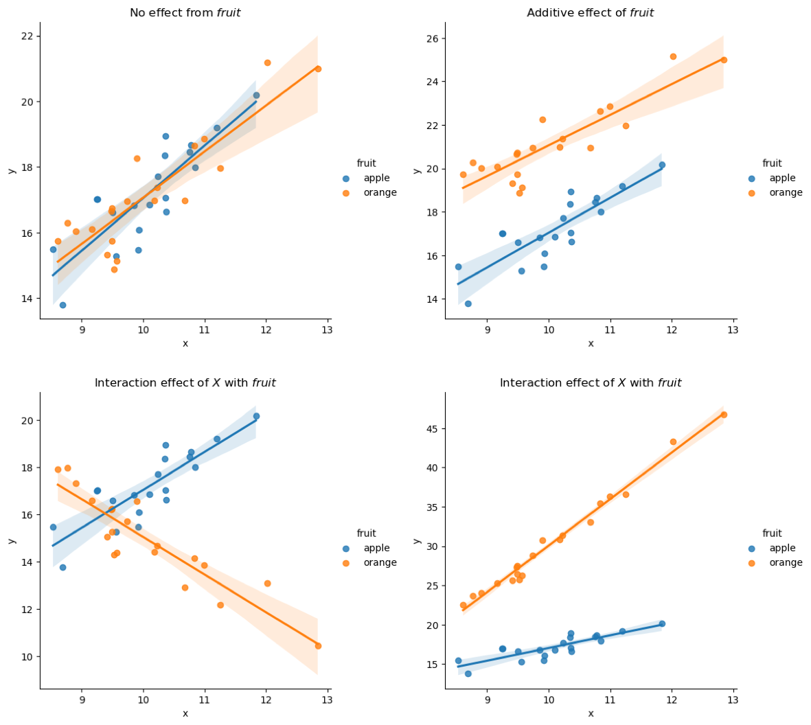
Here we have four different examples, the top two have no interaction effect, but additive effect as seen from earlier is observed in the plot on the top right. Bottom two plots are examples of interaction effect, where \(fruit\) depend on \(X\) and each fruit have a different coefficient as a result; This can be thought of the same as before where we have “two” models in one, but the interaction term within model would provide the statistical analysis to let us know that they are significantly different. It could also be done with a continuous variable where for example but it just makes it harder to visualise.
The visualisation shown above gives good understanding of interaction effect and much more straightforward, but this is limited to categorical predictors. In order to make it more general, we can use the following equations to compute the marginal effect due to interactions:
for marginal effect of \(X_1\) on \(Y\), holding \(X_2\) constant
\begin{equation} \frac{\partial Y}{\partial X_1} = \beta_1 + \beta_{1,2} X_2 \end{equation}
or for marginal effect of \(X_2\) on \(Y\), holding \(X_1\) constant
\begin{equation} \frac{\partial Y}{\partial X_2} = \beta_2 + \beta_{1,2} X_1 \end{equation}
The interpretation is just as before the \(\beta_1\) is effect per unit of \(X_1\) while other \(\beta\) is kept constant, but if \(X_2\) is not zero, and there is an interaction, the new effect of \(X_1\) would be \(\beta_1 + \beta_{1,2}X_2\). The \(\beta_{1,2}\) is the interaction effect, and its impact changes per unit of \(X_2\), and in the event of categorical predictors, it would mean the effect on the presence of the other variable.
Model Building Process
In SLR, I highlighted \(R^2\) as the metric to know if the model is “correct” or useful. This metric is also applicable for SLR, however, as mentioned above we can’t merely rely on a high \(R^2\) alone in deciding a good model, and to visualise it. When it comes to MLR, visualising it can be challenging as the number of dimensions have increased. Therefore we would now need to rely on other metrics to inform us if our MLR model is “correct”; these are AIC, BIC and log-likelihood, all these information are provided in the output from statsmodel shown above when you execute print(results.summary()), located just below R-squared value.
Stepwise Regression and Best Subset Regression
“Stepwise Regression” and “Best Subset Regression” are variable selection methods employed to build a model when faced with multiple variables. The idea is to select the “best” variables to go into the final model, which is not dissimilar to the idea of feature selections in machine learning.
Briefly Stepwise Regression: From a set of candidate predictor variables, they are added and removed to the model in a stepwise manner into the model, until there is no justifiable reason to add or remove anymore. The ‘reason’ can be determined by you using any of the statistical metric, for example p-value can be used, where we would examine if the added predictor would generate a ‘significant’ p-value, if not it can be removed. Or if addition of it would reduce another predictor’s significance and so on.
Briefly Best Subset Regression: From a set of candidate predictor variables, we would want to select the best subset that meets a given metric, for example \(R^2\) or mean-squared error. So this is basically done by testing all possible combinations of predictors and going through each model’s outcome. One extension of this method is to cross-validate using train-test dataset. This is done by splitting the dataset into training and test set, e.g. 70% samples are used for training, then we use the remainder 30% to test how well the selected predictor variables work on it. We can use this to pick the set of predictors that produces the lowest MSE on the test set. n
Personally, these two aren’t approaches I would use, in fact there are some people quite against these approaches; as these methods are running multiple tests hoping for the best. In my opinion, when building model having domain knowledge is always preferable. For example in the stepwise method, if addition of one variable increases p-value of another variable, this means there is possible confounding or correlation that requires more thought in the model building process. That said if interested, I found my old implementation of this two algorithms when I was learning them and have placed them in the notebook, if you are interested you can have a look and clean it up yourself if preferred.
Model Comparison
Aside from using the above metrics alone, another way to make sure model is useful or ‘correct’ after adding a variable or even an interaction effect is to perform model comparison that can be passed through a statistical test to generate a everyone’s favourite p-value. There’s two options for this:
- General Linear F test/ANOVA
- likelihood-ratio test (LRT)
But the core idea is the same, which is, we build two models:
i) a ‘full model’ including all variables/interaction of interest,
ii) ‘reduced model’ or ‘restricted model’ with the extra variable/interaction removed.
Then we compare it statistically, and decide which model to keep. This statistic is done with F-distribution for F-test or chi-squared distribution for LRT. The null hypothesis here is that the reduced model is better, therefore a ‘significant’ p-value indicate the full model (extra variable/interaction) is better. Better can be rephrased as explain the data/Y better.
The following example code is how you would perform a LRT:
### extract log-likelihood of fitted models
# where fullmodel is statsmodel object with full model fitted (after running .fit())
full_llf = fullmodel.llf
# as above but for reduced model, e.g. one variable less
reduced_llf = reducedmodel.llf

### ratio, but since it is log-transformed we can take the difference
likelihood_ratio = 2 * (full_llf - reduced_llf)

### take degree of freedom (dof) from models to be used in the stats calculation later
full_dof = full_llf.df_model
reduced_dof = reduced_llf.df_model

dof = full_dof - reduced_dof

### compute the p-value
# we use scipy for the statistics function
from scipy import stats
p = stats.chi2.sf(likelihood_ratio, dof)
Data Transformation
When your model fails to meet the LINE assumption, there is one solution, that is to transform your data. However, this is not a definite cure, after data transformation, you would still have to run the same assumptions check as before, as you have a new dataset.
The general rule is if you have:
- linear assumption violated, you transform \(X\).
- normalilty or equal variance assumption violated, you transform \(Y\).
- and if you were wondering, when independence assumption is violated, you have to use a different model, e.g. time series model if it is dependence due to time.
The options for transformations (and the Python code) are:
For non-linear variables (to make linear):
- logarithm
np.log(X)
- inverse
1/X
- exponential
np.exp(X)
For variables that are non-normal and have unequal variance:
- square-root
np.sqrt(Y)
- inverse
1/Y
- arcsin
np.arcsin(Y)
REMEMBER to store your newly created variables
Alternatively, there is a well-known method for data transformation that tries to make your dataset meet the assumptions, and it is the Box-Cox method. This is included within the scipy package.
## import
from scipy.stats import boxcox
## transform
transformed = boxcox(x)
Polynomials
Another transformation that can be used for when data is non-linear is the polynomial regression/transformation. To perform a polynomial regression, we bring variable up in power, for example this is a second order polynomial:
\begin{equation} Y=\beta_0 + \beta_1 X + \beta_2 X^2 \end{equation}
And we don’t have to stop at just second order, we can go up _n_th order polynomial.
\begin{equation} Y=\beta_0 + \beta_1 X + \beta_2 X^2 + \beta_3 X^3 + … + \beta_n X^n \end{equation}
But of course, do not go too crazy with the polynomial, p vs n still applies, one extra degree polynomial is one extra variable in the model.
What happens when we do this transformation? The following plots gives an example of the transformation in increasing order from left to right.
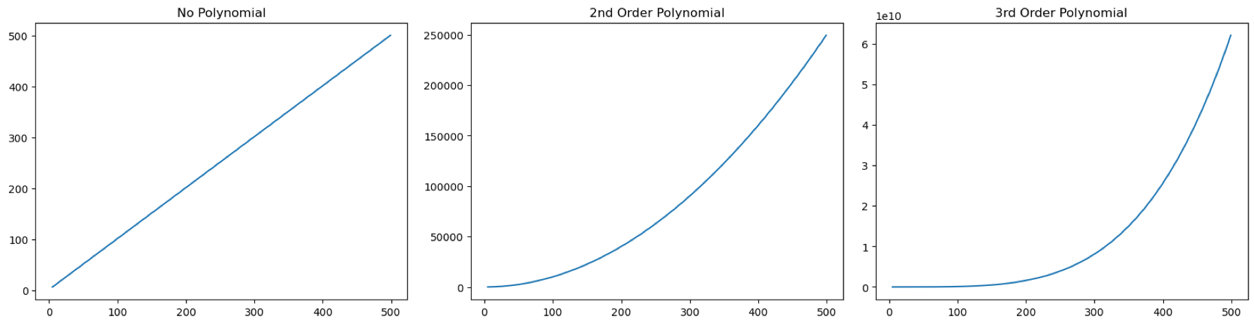
As I have mentioned many times before, always visualise your model. After initial visualisation you notice that your data points are non-linear, you can apply polynomial transformation, you should visualise it again to see that it is actually fitting your data well (as well as the \(R^2\) after fitting).
There is another known method for dealing with non-linear data, which is b-splines, but this method is rather advanced so I’ll be leaving this one out.
So… it might be obvious, all these transformations would change the previous simple interpretations. In fact, I don’t even know how to interpret them, but in my attempt to learn, my google found me this post that explains interpretating log-transformed dataset.
Beyond Linear Regression
At the start of this post, I called linear model the ‘swiss-army knife’ of models, not just because of all its applications and versatility granted from data transformations above, but also for its generalization on the type of data it can model. For those that took basic stats course would know the examples I have been giving are modelling only continuous data, but there are other kinds of data such as discrete, categorical and ordinal. In my MLR example, I talked about categorical data as an independent variable, but this can also be modeled as a dependent variable. To achieve this with linear model, we rely on link function to transform the outcome into a range between 0-1 and we can further dichotomise it into a categorical outcome by choosing a cutoff e.g. 0.5 to split into 0/1. When dealing with binary outcome, this is a simple _logistic regression_, and the equation is the following:
\begin{equation} Y\frac{1}{1+e^{-(\beta_0 + \beta_1 X)}} \end{equation}
The core concepts learned above are mostly transferable, most importantly the interpretation have changed. Those familiar with probability would know we are now dealing with log-odds, the \(\beta\) is the estimated increase in the log odds of the outcome per unit increase in the value of the X. To make it easier to understand, we can use transform \(\beta\) with the exponential function \(e^{\beta}\) in order to obtain the odds ratio associated with a one-unit increase in the X.
What is odds ratio (OR)?
Every unit increase is ‘OR’ many times more likely to to have the outcome. E.g. :
- if OR is 4, every unit increase is 4 times more likely to have the associated outcome.
- if OR is < 1, means the outcome is less likely to occur.
- if OR=1, there is no increase or decrease in likelihood of outcome, i.e. no association between X and Y.
Sometimes \(R^2\) is not computed, but usually a pseudo \(R^2\) is provided which provides a similar interpretation, this is also visible in the model.summary() function.
To build logistic model, I recommend to use the GLM function in statsmodels over the Logit function (which is the logistic regression function in statsmodels). Example code:
## usual formatting of y/X data for statsmodels
X = sm.add_constant(df.X)
y = df.y

## creating and fitting model
model = sm.GLM(y, X, family=sm.families.Binomial())
results = model.fit()

## with formula
model = smf.glm(formula="y ~ X", data=df, family=sm.families.Binomial())
results = model.fit()

## all other principles from before applies.
Generalized Linear Model
So what is this GLM that I prefer over Logit? GLM stands for generalized linear models, which is a this modelling framework that extends regression models to include many more data types than just continuous, and the Binomial version I chose is used for categorical outcomes (Y). For other ‘families’ of outcome that can be modelled, please visit this link which is extension through link functions.
Linear Mixed Effects Model
This is a variation of modelling that allows us to model dependent data (which violates one of the assumptions) that are generated from longitudinal data, i.e. samples that are collected over time multiple times (aka repeated measures). For example studying someone’s exercise and diet, you would have multiple observations on their weight, calories burned and food intake. This is where linear mixed effects model come in. Please follow the link to learn more on this as this is an advanced subject. In brief, instead of modelling all the parameters as fixed effects, it would can model some parameters of interest as random effects. And this fixed vs random is basically, maximum likelihood point estimate for fixed and a probabilistic estimation for random.
Alternatively, follow this blogpost for useful visualisation example as well as more explanation, but in with example code written R.
Time series model
Another advanced modelling method to deal with repeated observations over time is known as time-series analysis, and this is done with an autoregressive models. Difference of this method compared to mixed effects is that the model assumes/expects there is a trend/pattern over time that can be studied and predicted/forecasted.
Survival analysis
Another thing we can learn from tracking things over time, is when would an event happen, classically, this would be death, which is why this field of study is known as survival analysis. Regression can be extended to perform surival regression for use in survival analysis.
Causal Inference
The age old wisdom “correlation does not imply causation”. The field of study to determine causality is known as causal inference. And within this field are many different approaches, and linear model is employed in some of them that I know of. For example with directed acylic graphs, it involves an extra instrumental variable, Z, on top of X and Y. This involves the use of two-step linear model
And more…
There are more extensions in linear models that I have not listed because I am not familiar or even aware of their existence. But once you have a strong foundation within linear model alone, you can expand beyond it.
Summary
Linear model is a class of statistical method that can be used to model many things in a ‘general’ manner. This general-ness can be expanded through data transformation such as polynomial transformations and interaction models as well as use of link functions. Its use is found in many applications with two popular python packages supporting two specialised use case, which are statsmodels for hypothesis testing and scikit-learn for machine learning/prediction modelling. I cannot stress enough on the ‘generalness’ linear model, as Richard McElreath puts it, this is a geocentric model for statistics, while it is not accurate, it is still very useful. Even if most data in the world is not 100% linear or Normally distributed, linear model still can be applied. This is why it is found in all fields of research.
Disclaimer: This whole post may feel very heavy in content, but it is still a crash course where some things are overlooked. So don’t be surprised if there are still things that you do not understand when reading other literature on this subject matter. But I hope this gives you enough understanding to read a textbook and quickly fill in the blanks for yourself.
Appendix
Statistical Semantics/Glossary
Useful statistics semantics in case you want to venture out and read more on your own
Population model/statistics/parameter
- The wonderful imaginary optimal true model with parameters that accounts for every single sample available within the population being studied, such as the whole world or a given country, etc, which is often not known.
Estimated/Sample model/statistic/parameter
- The model built/estimated from limited (not all) samples of the population, which is what we really have, hence all the nuance calculations to include confidence interval and standard error etc.
Population vs sample is an important distinction. For example, we are studying the height of dwarves, we would only be able to measure (sample) 500 of their height. From this 500 measurement we can determine the sample mean, where mean is the model parameter. That is we know the mean of the samples measured but not true mean of the dwarf population being studied. Which is why confidence intervals are often included in the reporting of parameters, to state that we are 95% confident sample mean is the (true) population mean.
Degree of freedom (DOF)
- Not directly related to linear models, but an important factor in all statistical models. DOF is the number of ‘information/observations’ in the data that are free to vary when estimating statistical parameters. Usually
DOF = N - P, where N is the number of observations/samples available, and P is the number of a parameters being estimated. This is an important information because if DOF is less than or equals to 0, no p-values can be computed, therefore P cannot be more than N.
Independent and Dependent Variable
In case you skipped prologue, there are field specific synonyms to independent/dependent, which is detailed in this wiki page.
Effect size
For Linear Models, the coefficients are the effect sizes of the phenomenon being studied.
Close Form Solution
An oversimplification is that the equation can be solved analytically. That is we can move the variables around and we can compute the solution for a variable of interest easily.
E.g. in SLR we have simple y = b*x + c, if we know values of y/x/b. We want to solve for c, we just rearrange the equation to c = y - b*x, and put in the corresponding values to solve for c.
Log-likelihood
A likelihood of a given model is a measure of how ‘likely’ or ‘probable’ this model is in generating the given data. I say ‘given model’ because this is a statistical term that can be applied to any statistical models. As this explanation suggests, this can be used to decide how useful the model is, and the higher the value the better (more likely) the model. Log transformation on the model’s likelihood function would give you the log-likelihood. If you would like to know more on linear regression’s log-likelihood function, please follow this link.
Relevant Formulas
- mean of X/Y \begin{equation} \bar{x}/\bar{y} \end{equation}
- predicted Y \begin{equation} \hat{y} \end{equation}
- Intercept \begin{equation} \beta_0 = Y - \beta_1 X - \epsilon \end{equation}
- Regression coefficient \begin{equation} \beta_1 = \frac{\sum(x_i - \bar{x}) (y_i - \bar{y})}{(x_i - \bar{x})^2} \end{equation}
- Residuals \begin{equation} resid = y_i - \hat{y} \end{equation}
- Sum of squared residuals aka Sum of squared errors (SSE) \begin{equation} SSE = \sum(y_i - \hat{y})^2 \end{equation}
- Mean-squared error (MSE) \begin{equation} MSE = \frac{\sum(y_i - \hat{y})^2}{n-2} \end{equation}
- Akaike information criterion (AIC) \begin{equation} AIC = n \cdot ln(SSE) - n \cdot ln(n) + 2p \end{equation}
- Bayesian informaiton criterion (BIC) \begin{equation} BIC = n \cdot ln(SSE) - n \cdot ln(n) + p \cdot ln(n) \end{equation}
- n is sample size,
- p is number of parameters,
- ln is natural log.