
Yap Chuan Fu
Research Associate at The University of Manchester. I enjoy solving problems using computers and mathematics.
Bayes Classifier for Hackers
PyMC3 Crash Course - 10 min read
Published Apr 30, 2021
tldr; this post will cover usage of PyMC3 (python package) for building a (generative) model and classifying data in supervised manner.
DISCLAIMER: Hacker here does not mean Mr. Robot-esque hacking where you break into systems, sorry to disappoint if you came here wanting to break into systems with Bayes models. Rather, hacker here refers to someone whose natural approach to solving problems is to write code. E.g. simulating probabilities rather than calculating it (as it’ll be shown here) or performing tasks by automating it with code. An example of ‘way of the hacker’ is demonstrated in this talk, where he demonstrates we can replace t-test with a hack.
Motivation of the post
When people talk about machine learning, people always think/mention linear regression, random forest, support vector machines and neural network as that is often the entry point for people into these field, and the gateway tool for machine learning for python users is often scikit-learn. This was definitely the case for me, and in my continued pursuit to learn more on this field, I have come across the wonderful tool that is Bayesian (Probabilistic) Model, which I’ll be sharing in this post how to use it. The motto here is “If you can code you can do bayes modelling” (results may vary). For the mathematical purist, feel free to click away now in order to avoid aneurysm for such blasphemy.
In case the disclaimer wasn’t clear, this post will condense/avoid the maths behind it, and dive right into how to use the tool PyMC3 with the focus on using it for naives bayes classification. None of the mechanisms that make the inference engine run will be discussed, idea of this post is to get you to use it and love it and become interested enough to learn it to better debug your models. This is the same concept of getting you to drive your car without knowing how it works, and once you have fallen in love with the idea of cars, you’ll become a car person (not transformers) and learn everything bout it on your own.
PyMC3 is probabilistics modelling package in python powered by theano. There is a wikipedia page listing all the probabilistic programming options out there in case PyMC3 isn’t for you.
Below is the structure for this post, feel free to click to the section that is of interest. Let’s get started.
Table of Contents
- EDA
- Explore the dataset and understand what we are working with. We are working with classic Iris dataset, if you are familiar with it, you can skip this section.
- Building the Model
- Brief run down on the model being built and the code necessary to build a classifier to predict Iris flower species.
- Testing the Model
- Evaluating our model, and comparing against maximum likelihood version.
- Thoughts
- Thoughts on the method, such as its advantages/limitations and further reading.
- Glossary
- At any point you come across any words you don’t understand, here is a brief explanation.
But first, as you would with any jupyter-notebook or python scripts, import all the things~!
import pandas as pd
import numpy as np
## for plotting
import matplotlib.pyplot as plt
import seaborn as sns; sns.set()
## pymc the bayesian model tool
import pymc3 as pm
import theano.tensor as tt
import theano
## ml tools
import sklearn.datasets as data
from sklearn.model_selection import train_test_split
from scipy.stats import multivariate_normal, norm
from sklearn.metrics import accuracy_score, roc_auc_score
In case you tried to replicate some things and get drastically different results, here are the versions:
pandas=='1.2.4'
numpy=='1.20.1'
pymc3=='3.9.3'
scikit-learn=='0.24.1'
theano=='1.0.4'
Exploratory Data Analysis (EDA)
Load the data first from scikit-learn’s dataset module and check the dataset feature count and total number of targets.
X = pd.DataFrame(data.load_iris(as_frame=True)['data'])
y = pd.Series(data.load_iris(as_frame=True)['target'])
print(X.shape, y.unique().shape)
(150, 4) (3,)
Now we know there is total of 150 samples, 4 features, and 3 targets. As all good EDA should do, we should visualise our data. With only 4 features we can easily perform pairplot to see how each features correlate.
iris = X.copy()
iris['target'] = y.map({0:'setosa', 1:'versicolor', 2:'virginica'})
pplot = sns.pairplot(iris, hue="target")
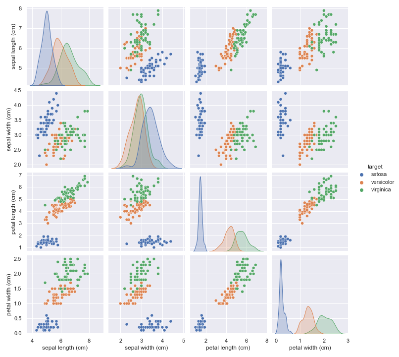 The plot shows us that setosa flower is nicely separated from versicolor and virginica, if thats all we care about, a simple linear model would suffice. Separating versicolor from virginica would not work with linear model.
And below is the distribution of the classes and fortunately there is no class imbalance issue.
| target | |
|---|---|
| setosa | 50 |
| versicolor | 50 |
| virginica | 50 |
Buiding the Model
To build our model, I’ll be modelling the dataset with Multivariate Gaussian distribution for the features. The idea is that each Iris flower type’s features are represented by a Multivariate Gaussian distribution, and our models will learn the distribution (information) of said features.
\begin{align} X \sim \mathcal{N}(\mu,\,\Sigma)\,. \end{align}
the classification will be done with \begin{align} P(c|X) ~ P(X|\mu, \Sigma) * P(c) \end{align}
where…
- c = classes
- X = features’ values
- \(\mu\) = mean/centre
- \(\Sigma\) = covariance
Bayesian inference
In bayesian fashion I’ll be estimating the parameters of the distributions of each classes. Meaning I’ll be building 3 Multivariate normal distribution models (one for each classes) like so:
\begin{align} P(\mu, \Sigma|X) = \frac{P(X|\mu, \Sigma) * P( \mu, \Sigma )}{P(X)} \end{align}
where the priors \(\mu\) and \(\Sigma\) will be modeled with, exponential and LKJCholeskyCov distributions respectively.
** follow this link for more information on why this distribution is used instead of Wishart. **
Now to actually build the model
def iris_model(X, y):
    K = len(y.unique())
    with pm.Model() as model:

        for c in y.unique():
            ## setting up priors for the model
            µ = pm.Exponential("µ{}".format(c), lam=1, shape=4)
            packed_L = pm.LKJCholeskyCov('packed_L{}'.format(c), n=4,
                                 eta=2., sd_dist=pm.HalfCauchy.dist(2.5))
            L = pm.expand_packed_triangular(4, packed_L)
            cov = pm.Deterministic('cov{}'.format(c), L.dot(L.T))

            ## the likelihood of the model is defined, which is where we input the data for the model to learn the parameters distribution with "observed"
            obs = pm.MvNormal('mvgauss{}'.format(c), μ, chol=L, observed=X[y==c])

    return model
Here I have wrapped model into a function to make it easier to call the model for whatever purpose. For those familiar with scikit-learn, this code block is analogous lm=LinearRegression() if you have to write the y=mx+c yourself. What each lines does is explained with comments within the code block. But for PyMC3, we typically set up priors (the parameters of the model usually, as it would be turned into posterior Bayesian style) and likelihood (where you define datapoint input, much like scikit-learn’s fit function, but the fitting is not done yet in this case).
This particular model definition is only for learning the Iris dataset. Unfortunately, there is no one size fit all model like those scikit-learn. If you would like to model other dataset with PyMC3, you would need to define the model yourself with the distribution that best describes your data.
With the model defined, we can compile it and check the graph visually to see if it is defined properly
## good ol train test split for model evaluation later
X_train, X_test, y_train, y_test = train_test_split(X, y, test_size=0.2, random_state=42, stratify=y)
pm.model_to_graphviz(iris_model(X_train, y_train))
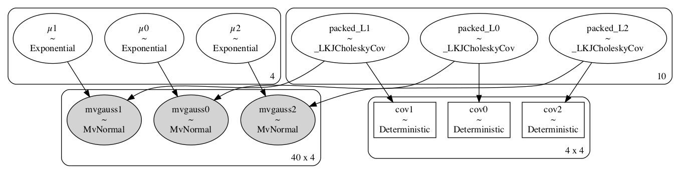 We can see we built the model correctly with the
 for loop, resulting in 3 models, 1 for each class.
Now we will fit the model by running the Bayesian inference engine with the following code.
with iris_model(X_train, y_train):
    trace = pm.sample(random_seed=42)
This small model should take a few minutes to run, there would be some deprecation errors popping up but it will still run fine. PyMC3 has a nice progress bar to inform users on the sampling progress as well.
Checking convergence
One thing to always do in Bayesian computational modelling is to check if the model converged. A quick convergence test is with the rhat value which we can check with the following, and it should be value of 1 for good convergence.
print(pm.summary(trace)["r_hat"].head().to_markdown())
| r_hat | |
|---|---|
| µ0[0] | 1 |
| µ0[1] | 1 |
| µ0[2] | 1 |
| µ0[3] | 1 |
| packed_L0[0] | 1 |
We can also check the final result of the fit with
pm.traceplot(trace)
The column on the left is the distribution for the estimated parameters, and the right column is the trace plot, which is the random samples drawn to form the distribution (default sampling size is 2000). Sampling means drawing random samples from the distribution from our model. Much like scipy’s norm.rvs(size=1000) which is drawing 1000 random samples from a normal distribution.

Naive Bayes
Since the model have converged, we can do quick predictions with Naive Bayes approach.
This is done by computing the probability density for a sample’s feature values given the fitted parameters. We do this using all 3 classes’ parameters, the class that gives the highest probability density amongst the 3 would would be chosen class for the sample.
That is, when classifying sample x…
\begin{align} argmax[{ P(x|\mu_1, \Sigma_1) ,P(x|\mu_2, \Sigma_2), P(x|\mu_3, \Sigma_3)}] \end{align}
Here is a simple code block to do this, the reason we have a for loop with 2000 iterations is to compute them for each of the 2000 samples. There is probably a vectorize way to avoid the for loop, but I have yet to experiment with that.
def naivesbayes(X):
    mvnorm_pdf = multivariate_normal.pdf
    samples = X.shape[0]

    c1_p = np.empty((2000, samples))
    c2_p = np.empty((2000, samples))
    c3_p = np.empty((2000, samples))

    for i in range(2000):
        c1_p[i] = mvnorm_pdf(X.values, mean=trace["µ0"][i,:], cov=trace["cov0"][i,:,:])
        c2_p[i] = mvnorm_pdf(X.values, mean=trace["µ1"][i,:], cov=trace["cov1"][i,:,:])
        c3_p[i] = mvnorm_pdf(X.values, mean=trace["µ2"][i,:], cov=trace["cov2"][i,:,:])

    y_pred = pd.DataFrame()
    y_pred["0"] = c1_p.mean(0)
    y_pred["1"] = c2_p.mean(0)
    y_pred["2"] = c3_p.mean(0)

    y_pred = y_pred.idxmax(axis=1).astype("int64")

    return y_pred
Testing the Model
Now that we have the converged models and have a way to make predictions with it, we should evaluate it. Here we use scikit-learn’s accuracy score metric function.
nbtrain = accuracy_score(y_train, naivesbayes(X_train))
nbtest = accuracy_score(y_test, naivesbayes(X_test))
print(nbtrain, nbtest)
0.975 1.0
This output indicates the model is generalizing well.
Another approach to building models like this is to do it with maximum likelihood approach which is done by taking the mean and covariance without caring bout its dispersion and use that as model parameters. Scikit-learn has a module for this, we can implement that and see how it performs.
from sklearn.naive_bayes import GaussianNB
model_sk = GaussianNB(priors = None)
model_sk.fit(X_train,y_train)

mletrain = accuracy_score(y_test, model_sk.predict(X_test))
mletest = accuracy_score(y_train, model_sk.predict(X_train))
print(mletrain, mletest)
0.967 0.958
It too does pretty decently, as most model should with the Iris dataset.
Prediction probability
My previous code block for prediction gives a hard prediction without the probabilities, which would not really do in the probabilistic modelling scene! Below is a code block for prediction probabilties which would allow us to score our model with area under roc.
def NBpredict_proba(X):
    mvnorm_pdf = multivariate_normal.pdf
    samples = X.shape[0]

    c1_p = np.empty((2000, samples))
    c2_p = np.empty((2000, samples))
    c3_p = np.empty((2000, samples))

    for i in range(2000):
        c1_p[i] = mvnorm_pdf(X.values, mean=trace["µ0"][i,:], cov=trace["cov0"][i,:,:])
        c2_p[i] = mvnorm_pdf(X.values, mean=trace["µ1"][i,:], cov=trace["cov1"][i,:,:])
        c3_p[i] = mvnorm_pdf(X.values, mean=trace["µ2"][i,:], cov=trace["cov2"][i,:,:])

    y_proba = np.empty((samples, 3))

    for i in range(samples):
        pred = np.vstack((c1_p[:,i],c2_p[:,i],c3_p[:,i])).T
        pred = np.argmax(pred, axis=1)
        c1 = len([a for a in pred if a == 0])/2000
        c2 = len([a for a in pred if a == 1])/2000
        c3 = len([a for a in pred if a == 2])/2000
        y_proba[i] = np.array([c1, c2, c3])

    return pd.DataFrame(y_proba)
Now to score our model
roctrain = roc_auc_score(y_test, NBpredict_proba(X_test),multi_class="ovo")
roctest = roc_auc_score(y_train, NBpredict_proba(X_train),multi_class="ovo")
print(roctrain, roctest)
1.0 0.9995
Voila~!
Thoughts
This concludes our journey in using PyMC3 for building a generative model for classifcation, if you made it to the end, I hope you enjoyed the post and hope this encouraged you to explore more on using this method/tool. There are more advanced usage of bayes modelling which are detailed in tutorial and examples pages of PyMC3 website, one of these “advanced” usage that I particularly enjoy is hierarchical model, maybe I’ll write a post of this as well. Additionally, there are more sophisticated approaches than Naive Bayes when building probabilistic model for classification which involves use of a loss function to help make the predictions. The loss function is something I am still learning myself, when I have that figured out, I’ll likely write a post on that.
Distributions
One thing to note is that I mention the use of this and that distributions. Use of distributions is not set in stone, nor is this something you should (even if you can, I know I have been guilty of it) mess around for achieving the best results. One way to think about what distributions to choose is to understand how the data is generated, simple starting point is discrete vs continuous, should the values always be positive or are negative values possible. If you are comfortable with reading mathematics you can check out this post which would introduce you to the different distributions you can employ, or head on over to PyMC3 docs and hack around it. I know I said you shouldn’t mess around and at the same time encouraged messing around. My apologies for the confusion, in all seriousness this post’s take-away message is that you most definitely should just mess around, as you can learn quite a bit by doing!
Frequentist vs Bayesian
I am not here to pick a side as I am a pragmatist, if it works it works. But this short paragraph is to clarify for some what are the differences, as I was confused when I first started learning this.
To explain this briefly, I’ll use the example of linear regression model:
- Frequentist approach of building this model would give point estimate(s) for the parameter(s) and confidence intervals, where point estimate means single value. E.g. one coefficient, one value.
- Some would be familiar with the term maximum likelihood, that is to say, you obtain the best possible value for the parameter.
- Bayesian appraoch of building this model would generate distributions for the parameters. E.g. one coefficient has a range of values with varying probabilities for the values.
- That is to say in Bayes, everything is distribution, the model is distributions, the inferred/optimised parameters are distributions (you can fix some values in the model building if desired).
If the above didn’t explain any of it to you clearly, the best explanation I have ever read is by Jake VanderPlas from his series of post regarding this, and the best line regarding frequentism vs bayesian from his posts is the following:
- Frequentist treat parameters as fixed, data as random variables
- Bayesian treats parameters as random variables, data as fixed.
Semantics
Some may have noticed I used Bayesian and Probabilistic model interchangebly, they are more or less the same thing, mathematical semantics is always annoying for me personally, but for all intents and purposes, they are the same. Reason for this is output of Bayes models are probabilistic as they generate a distribution, which we can sample from. Another word that is used to describe Bayes model is statistical model, if you come across this term, it can mean Bayes model or it may not. From my understanding, statistical model is a family of mathematical models, and Bayes models is one of them, so calling Bayes model statsitical/mathematical model is correct, but assuming statistical model is Bayes model may not always be correct.
To sum up, Bayes model is a type of statistical model, and statistical models are types of mathematical models.
Advantages
Bayes model are not just limited to classifying, but it can also use the inferred parameters to generate data close to the dataset it learned from. Additionally, the parameters within can be scrutinized for further analysis if desired, given your understanding on the model.
Disadvantage
One thing I have encountered is that, as the dimension of data increases, the performance of the model decreases.
Glossary
- Generative Model - A model that can be used to generate data, as well as classify things, the inferred parameters can also be used for various things. It is typically a probability model with distributions etc.
- Machine Learning - Algorithm/Maths that learns the pattern of the data.
- Probabilistic Programming - Tool/language for building probabilistic models.
- Inference Engine - The machinery that makes the inference, where inference means obtaining (inferring) the parameters behind the distribution/model.
- Theano - I want to say it is NumPy on steroids, I don’t know enough to comment beyond that.
Notebook link
Click here for the jupyter-notebook that contains all the code used here.